WHAMP Tutorial for Plasma Wave Dispersion Analysis
A comprehensive guide to using WHAMP for studying plasma instabilities with Python automation
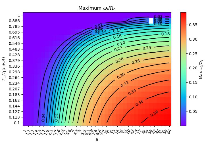
NOTE: Guide for using python wrapper for WHAMP (Waves in Homogeneous Anisotropic Magnetized Plasma). The example that is considered is parallel firehose instability.
Introduction to WHAMP
WHAMP is a Fortran code originally written by Kjell Rönnmark that calculates general wave dispersion relations in plasmas

The key physics behind WHAMP involves solving the dispersion relation:
\[\det(\mathbf{K}) = 0\]where $\mathbf{K}$ is the wave operator matrix that depends on the plasma parameters, wave frequency $\omega$, and wave vector $\mathbf{k}$. For each set of plasma conditions, WHAMP finds the complex frequency $\omega = \omega_r + i\omega_i$ where:
- $\omega_r$ is the real frequency (wave propagation)
- $\omega_i$ is the imaginary frequency (growth/damping rate)
The parallel firehose instability occurs when $T_\perp < T_\parallel$ (temperature anisotropy $A = T_\perp/T_\parallel < 1$) and manifests as unstable modes with $\omega_i > 0$ propagating parallel to the magnetic field.
A good source for understanding parallel firehose instaiblity is the book
Setting Up the Environment
Clone the wrapper fork of the original WHAMP repository and navigate to the src directory:
git clone git@github.com:georgemilosh/whamp.git
cd src
Ensure you have the required dependencies and WHAMP compiled:
# Build WHAMP
make clean && make
We have made some small modification to the original WHAMP code to allow more flexibility in input parameters and integration with the wrapper
The project structure should look like:
whamp/
├── src/
│   ├── whamp_wrapper.py      # Python wrapper
│   └── whamp                 # Compiled executable
├── Models/
│   └── H17f3c               # Example plasma model
├── results/
│   └── (output files)
└── examples/
    └── parallel_firehose_sweep.ipynb
Setting up the plasma model
To set the physical model for WHAMP, you need to create a text file with the plasma parameters. The format is as follows:
# Model from Fig 5 of Hunana, P.; Zank, G. P. On the Parallel and Oblique Firehose Instability in Fluid Models. ApJ 2017, 839 (1), 13. https://doi.org/10.3847/1538-4357/aa64e3.
# Density values (m^-3) for 10 species
1.0e6 1.0e6 0.0 0.0 0.0 0.0 0.0 0.0 0.0 0.0
# Temperature values (eV) for 10 species
0.005  1e-8 0.0 0.0 0.0 0.0 0.0 0.0 0.0 0.0
# Loss cone parameter D for 10 species
1.    1.   1.0 1.0 1.0 1.0 1.0 1.0 1.0 1.0
# Temperature anisotropy A for 10 species
0.49    1.   1.0 1.0 1.0 1.0 1.0 1.0 1.0 1.0
# Loss cone parameter B for 10 species
0.0   0.0  0.0 0.0 0.0 0.0 0.0 0.0 0.0 0.0
# Atomic mass for 10 species (0=electron, 1=proton, etc.)
1.0  0.  0.0 0.0 0.0 0.0 0.0 0.0 0.0 0.0
# Drift velocity for 10 species
0.    .0  0.0 0.0 0.0 0.0 0.0 0.0 0.0 0.0
# Electron Gyrofrequency (kHz)
0.01986
# PZL parameter
0
# Ion to electron mass ratio
1836.1
We have added the possibility of having comments and the possibility to control the ion to electron mass ratio which was previously hardcoded to 1836.1. The file should be saved in the Models/modelname
Python Wrapper Implementation
The whamp_wrapper.py module provides three main functions for automating WHAMP simulations. Let’s examine the key components:
Reading WHAMP Output
read_whamp_output - The most critical function parses WHAMP’s output format. This function reads the WHAMP output text file and parses key parameters such as perpendicular and parallel wavenumbers (p, z), real and imaginary parts of the frequency (omega_r, omega_i), and electric field components. It uses regular expressions to extract these values from each line and returns a pandas DataFrame for further analysis.
Parameter Sweep Analysis
The most powerful feature is automated parameter sweeps. Here’s how to study the parallel firehose instability across different temperature anisotropies and plasma beta values:
read_whamp_automated - This code performs an automated parameter sweep for a plasma simulation using the run_whamp_automated function. It:
- Defines ranges for temperature anisotropy (a_values) and cyclotron frequency (c_values).
- Builds a sequence of command strings to set up and run simulations for each parameter combination.
- Adjusts the wavenumber scan range based on the anisotropy value.
- Executes the simulation sweep and saves results to a file.
Understanding WHAMP Commands
The command syntax follows specific patterns:
| Command | Description | Example Usage / Notes |
|---|---|---|
p0,1,-.1 | Set P range: start=0, end=1, step=-0.1 | Perpendicular wavenumber (descending) |
z0,2,.1 | Set Z range: start=0, end=2, step=0.1 | Parallel wavenumber (ascending) |
p0 | Set P fixed value | Parallel wavenumber (fixed value) |
f1e-4 | Set frequency guess | Initial frequency |
a2.0 | Set temperature anisotropy A=2.0 | $T_\perp/T_\parallel$ |
a(2)2.0 | Set anisotropy for second species | $T_{\perp,2}/T_{\parallel,2}$ |
c0.1 | Set electron cyclotron frequency c=0.1 kHz | Magnetic field strength |
pzfewa | Output format: p,z,f,e,w,a | Electric fields + wave parameters |
pzfewa(2) | Output format: p,z,f,e,w,a(2) | Electric fields + wave parameters |
For parallel firehose the following commands are used:
    a_values = np.logspace(np.log10(0.1), np.log10(1.0), num=20)  # logarithmically spaced between 0.1 and 1.0 inclusive
    c_values = np.logspace(np.log10(2*0.01986), np.log10(0.01986/4), num=40)  # logarithmically spaced cyclotron frequency
    f_values = [1e-1 for _ in range(len(c_values))]  # sweep over frequency
    commands = ['p0z0,1.5,-.1f1e-4', 'pzfewa']
    for c, f in zip(c_values, f_values):
        for a in a_values:
            commands.append(f'c{c}a{a}f{f}')
            if a > 0.8:
                commands.append('z0,.6,-.05')
            else:
                commands.append('z0,2,-.1')
            commands.append('p0z0,1,-.05')
    commands.append('S')
The intuition is to find a good initial guess for the frequency and initial wavenumber. The code will attempt to stay on the same branch while sweeping through p and z wavenumbers. If c or a are changed the code starts adjusting from again.
Data Analysis and Visualization
Once the parameter sweep completes, we can analyze the results by making sure that the right eigenmodes are selected, corresponding to the parallel firehose instability.
# Load and clean the data
df_raw = read_whamp_output('../results/parameter_sweep.txt')

# Filter out spurious high-frequency solutions
df = df_raw[(df_raw['omega_r'] <= 1e3) & (df_raw['omega_r'] >= -1e3)]

# Filter for right-hand circularly polarized modes (parallel firehose)
df = df[(df['EX_real']/df['EY_imag'] == 1) & (df['EY_real']/df['EY_imag'] == 0)]

print(f"Filtered data: {len(df)} points")
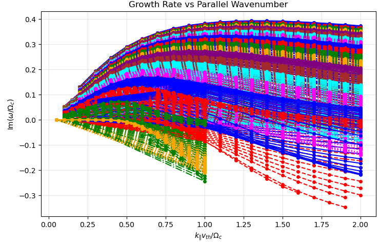
To make the figure in the beginning of the post, we can use the scripts found in the jupyter notebook.

Enjoy Reading This Article?
Here are some more articles you might like to read next: