Standard Nontwist Map
Both chaos theory and fractal have had contacts in the past when they are both impossible to develop and in a certain sense not ready to be developed. - Benoit Mandelbrot
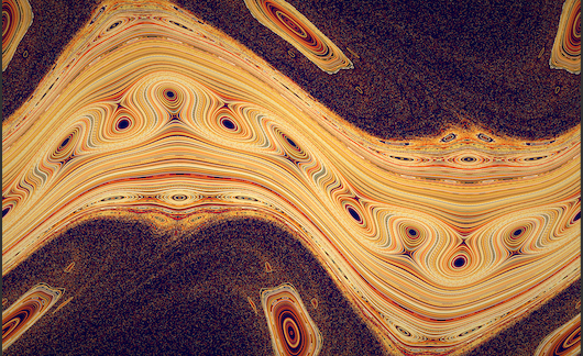
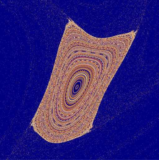
In this post I discuss how I made the figures that won the third place for visualization of science contest at the University of Texas at Austin where I did my PhD. The image is based on research produced many years ago on Nontwist maps by del-Castillo-Negrete and Morrison. These maps were developed to describe discretized low-dimensional dynamics that preserves areas under transformation and violates the so-called twist condition (see equation \eqref{eq:twist}). For more details on mathematical and physical properties see a review on Scholarpedia.. The model is rather abstract but it aims to provide understanding for chaotic transport and quasi-integrable systems. The equations descrbing the Standard Nontwist Map (SNM) are as follows
\begin{equation}\label{eq:SNM} \begin{aligned} &\overline{\mathrm{x}}=\mathrm{x}+\mathrm{a}\left(1-\overline{\mathrm{y}}^2\right), \quad(\text { modulo } 1)
&\overline{\mathrm{y}}=\mathrm{y}-\mathrm{b} \sin (2 \pi \mathrm{x}) \end{aligned} \end{equation}
with the non-twist condition
\begin{equation}\label{eq:twist} \frac{\partial \overline{\mathrm{x}}(\mathrm{x}, \mathrm{y})}{\partial \mathrm{y}} \geq \mathrm{c}>0 \quad \forall(\mathrm{x}, \mathrm{y}) \end{equation}
The map (equation \eqref{eq:SNM}) is iterated succesively, so one can think of points on it as Poincare Sections of map that could correspond to, say, points where magnetic field line pierces a page. The colormap is chosen for easthetical reasons, however, it does correspond to initial conditions (each color is locus of points that correspond to a given iteration). The continuous (orderly) points correspond to periodic orbits, whereas around we see lots chaotic orbits. When the control parameters \(a\) and \(b\) are varied the shape of the image changes significantly from completely integrable (straight lines) image to completely chaotic. Below we give maps for parameters that we found most aesthetically pleasing
1
2
3
4
5
6
7
8
9
10
11
12
13
 Graphics[
    a = 0.615; b = 0.4;
    data = Table[RecurrenceTable[{q[n + 1] ==
    Mod[q[n] + a (1 - (p[n] - b Sin[2 \[Pi] q[n]])^2), 1],
    p[n + 1] == p[n] - b Sin[2 \[Pi] q[n]],
    p[1] == RandomReal[{-0.5, 0.5}],
    q[1] == RandomReal[{0, 1}]}, {q, p}, {n, 1, 500}], {i, 1, 500}];
    AbsoluteTiming[ListPlot[data, PlotRange -> { {0,1} , {-0.5,0.5} }/,
    ImageSize -> Full, Axes -> False, PlotMarkers ->  {"\[FilledCircle]", 0.5},
    PlotStyle -> ColorData["SunsetColors"]/@
    (Range[0, Length@data]/Length@data), Background -> Darker[Blue, 0.5],
    ImageSize -> Full, PerformanceGoal -> "Speed"]
]


Enjoy Reading This Article?
Here are some more articles you might like to read next: