academic diagrams

This short blog is meant to provide some reference for making diagrams in LaTeX using TikZ&PGF package. While the manual is quite in-depth I decided to provide my own notes to give an introduction to the impatient.

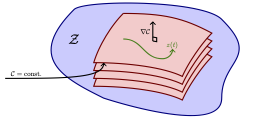
Below, I show a how to make this pretty diagram I created for my thesis Thesis 2018

Setting up TikZ

The details don’t matter very much in this post, but this object comes from noncanonical Hamiltonian formalism. The idea is to show how the phase-space is foliated by such Casimir leaves, which are functionals that constrain trajectories of the system. I wanted a blob describing the space I am in, \(Z\), as well as the pictures of the leaves and the trajectory.

First we have to load the appropriate packages that will be needed prior to using the tikz environement:

\documentclass{article}
\usepackage{graphics}
\usepackage{tikz}

\def\calc{\mathcal{C}} %Defining the mathematical symbol shortcuts
\def\calz{\mathcal{Z}}
%--------------------------------------% 

The remainder of the commands will go instide the tikz environment

%-- Main Document --------------------------------------------------
\begin{document}
  \begin{tikzpicture}[scale=1] % scale allows us to change the size of the diagram
      % tikz enviornment is here  
  \end{tikzpicture}
		
\end{document}

Creating the leaf

The main object of the diagram is the leaf itself. We will represent them by curved page-like sheets. First we will work on the contour lines of this sheet. To get a better idea we plot auxiliary coordinate axes This can be done via the following command. The \draw command creates the graphical object. To draw a line use – providing the initial and final coordinates on the left and the right respectively. The various options of the \draw environment can be specified in the brackets.

     \draw[step=.5cm,gray,very thin] (-1.4,-1.4) grid (1.4,1.4);
     \draw (-1.5,0) -- (1.5,0);
     \draw (0,-1.5) -- (0,1.5);

The coordinate axes can be seen the leftmost panel below.

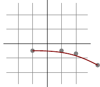
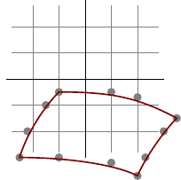
The next step is to draw the ouline of the sheet (mid-panel above). We start by drawing a line, which starts at \((-0.5,-0.25)\) and ends at \((1.75,-0.75)\). Because the line is epxected to curve we use controls command, and specify additional two points that control the trajectory (this is similar to bezier line in say Corel Draw). To make things more clear we also plot the inidividual points as circles. They are just a scafolding to be removed soon.

    \filldraw [gray] (-.5,-.25) circle (2pt)
     (.5,-.25) circle (2pt)
     (1,-.35) circle (2pt)
     (1.75,-.75) circle (2pt);
    \draw[draw=red!50!black,  thick] (-.5,-.25) .. controls (.5,-.25) and (1,-.35) .. (1.75,-.75);

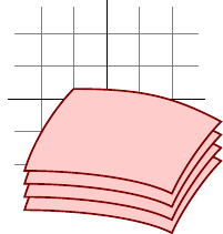
The rest of the sheet can be made likewise which is trivial. The nice thing about TikZ is that we can automatically clone the sheet once it is ready to create foliation via a for loop:

    \foreach \x in {-.2,0,...,.4}	
	\filldraw[fill=red!20!white, draw=red!50!black, ultra thick] (-.5,-.25+\x) 
		.. controls (.5,-.25+\x) and (1,-.35+\x) .. (1.75,-.75+\x)
		.. controls (1.5,-1+\x) and (1.15,-1.5+\x) .. (1,-1.85+\x)
		.. controls (.5,-1.6+\x) and (-.5,-1.5+\x) .. (-1.25,-1.5+\x)
		.. controls (-1.1,-1+\x) and (-.75,-.5+\x) .. (-.5,-.25+\x);

Subsequently, the trajectory and the perpendicular can be made. We just need to know how to draw arrows, together with a label.

    \draw[->,ultra thick] (0.25,-.55) -- +(90:.5) node[midway,left,scale=.5] {$\nabla\calc$}; 

To make a vertical arrow (perpendicular to the leaf) we can use

\draw[ultra thick] (0.25,-.55) -- ++(-10:.1)-- ++(90:.1)-- ++(170:.1);
					\node at (-1.75,-.5) [] {$\calz$};		

Here we have used ``++’’ command, which is based on relative coordinates (relative to the previous point). Otherwise absolute coordinate system is used. To make the green curving trajectory add the following line

   \draw[green!50!black, ultra thick,->] (0-.5,1/2-1) .. controls (1/2-.5,1/2-1) and (1/2-.5,0-1) 
        .. (2/2-.5,0-1) .. controls +(.555/4,0) and
		 +(0,-0.555/4) .. (2.5/2-.5,.5/2-1) node[very near end,above,scale=.5] {$z(t)$};

We also add a tooltip which specifies that the leaf is a Casimir leaf:

   \draw[->,ultra thick] (-3.5,-1.5) .. controls (-2,-1.5) and (-1,-1.5) .. (-1,-1.1) 
          node[very near start,above,scale=.5]{$\calc = const$.};

Exercise for a student:

Create the outline for the phase space (blue shaded region).

Extracting diagram-f1.pdf

This last paragraph is for those who want to extract a small image out of the pdf. The name of the file is diagram.tex and it can be made to extract a file by the name diagram-f1.pdf using a script

pdflatex --jobname=diagram-f1 diagram.tex